Getting Started with nestkit#
This notebook demonstrates the core functionality of nestkit - a rigorous nested cross-validation toolkit for scikit-learn.
What you’ll learn#
How to run nested CV for binary classification
How to inspect and interpret results
How to create basic visualizations
How to add probability calibration
How to add threshold optimization
How to run nested CV for regression with prediction intervals
Prerequisites#
pip install nestkit[plotting]
[1]:
import warnings

import matplotlib.pyplot as plt
import numpy as np
from sklearn.datasets import load_breast_cancer, load_diabetes
from sklearn.ensemble import RandomForestClassifier
from sklearn.linear_model import Ridge

from nestkit import NestedCVClassifier, NestedCVRegressor
from nestkit.plotting import (
    plot_calibration_curves,
    plot_calibration_improvement,
    plot_confusion_matrices,
    plot_inner_cv_heatmap,
    plot_outer_scores,
    plot_param_selection,
    plot_precision_recall_curves,
    plot_predicted_vs_actual,
    plot_prediction_intervals,
    plot_residual_qq,
    plot_residuals,
    plot_roc_curves,
    plot_score_stability,
    plot_threshold_comparison,
    plot_threshold_distribution,
    plot_threshold_sensitivity,
)

warnings.filterwarnings("ignore")

%matplotlib inline
plt.rcParams["figure.dpi"] = 100
1. Binary Classification with NestedCVClassifier#
We’ll use the breast cancer dataset (569 samples, 30 features, binary target) to demonstrate nested CV for classification.
Standard cross-validation conflates model selection with performance estimation, producing optimistically biased scores. Nested CV separates the two:
Inner loop - hyperparameter tuning on the outer training set
Outer loop - unbiased evaluation on the held-out outer test fold
[2]:
X, y = load_breast_cancer(return_X_y=True)
feature_names = list(load_breast_cancer().feature_names)
print(f"Shape: {X.shape}")
print(f"Classes: {np.unique(y)}, counts: {np.bincount(y)}")
Shape: (569, 30)
Classes: [0 1], counts: [212 357]
[3]:
ncv = NestedCVClassifier(
    estimator=RandomForestClassifier(random_state=42),
    param_grid={"n_estimators": [50, 100, 200], "max_depth": [3, 5, 10]},
    outer_cv=5,
    inner_cv=3,
    scoring="roc_auc",
    random_state=42,
)
ncv.fit(X, y)
[3]:
NestedCVClassifier(estimator=RandomForestClassifier(random_state=42),
                   inner_cv=3,
                   param_grid={'max_depth': [3, 5, 10],
                               'n_estimators': [50, 100, 200]},
                   random_state=42, scoring='roc_auc')
In a Jupyter environment, please rerun this cell to show the HTML representation or trust the notebook. On GitHub, the HTML representation is unable to render, please try loading this page with nbviewer.org.
Parameters
| estimator | RandomForestC...ndom_state=42) | |
| param_grid | {'max_depth': [3, 5, ...], 'n_estimators': [50, 100, ...]} | |
| search_strategy | 'grid' | |
| outer_cv | 5 | |
| inner_cv | 3 | |
| scoring | 'roc_auc' | |
| refit | True | |
| return_train_score | False | |
| return_estimator | True | |
| error_score | 'raise' | |
| n_jobs_outer | None | |
| n_jobs_inner | None | |
| verbose | 0 | |
| random_state | 42 | |
| callbacks | None | |
| pre_dispatch | '2*n_jobs' | |
| calibration_method | None | |
| threshold_strategy | None | |
| threshold_criterion | 'youden' | |
| threshold_beta | 1.0 | |
| cost_matrix | None | |
| min_recall | None | |
| calibration_cv | None |
RandomForestClassifier(random_state=42)
Parameters
| n_estimators | 100 | |
| criterion | 'gini' | |
| max_depth | None | |
| min_samples_split | 2 | |
| min_samples_leaf | 1 | |
| min_weight_fraction_leaf | 0.0 | |
| max_features | 'sqrt' | |
| max_leaf_nodes | None | |
| min_impurity_decrease | 0.0 | |
| bootstrap | True | |
| oob_score | False | |
| n_jobs | None | |
| random_state | 42 | |
| verbose | 0 | |
| warm_start | False | |
| class_weight | None | |
| ccp_alpha | 0.0 | |
| max_samples | None | |
| monotonic_cst | None |
2. Inspecting Results#
After fitting, ncv.results_ returns a ClassifierResults object with summary statistics, per-fold predictions, best hyperparameters, and generalization gap analysis.
[4]:
results = ncv.results_
results.summary_default_
[4]:
| metric | mean | std | ci_lower | ci_upper | median | iqr | |
|---|---|---|---|---|---|---|---|
| 0 | accuracy | 0.959618 | 0.028121 | 0.907243 | 1.011993 | 0.973684 | 0.043704 |
| 1 | balanced_accuracy | 0.955556 | 0.032409 | 0.895194 | 1.015918 | 0.969246 | 0.057960 |
| 2 | precision | 0.964525 | 0.032206 | 0.904540 | 1.024509 | 0.972603 | 0.043254 |
| 3 | recall | 0.971909 | 0.024452 | 0.926368 | 1.017450 | 0.985915 | 0.014280 |
| 4 | f1 | 0.967937 | 0.022510 | 0.926013 | 1.009862 | 0.979310 | 0.033333 |
| 5 | roc_auc | 0.990150 | 0.009537 | 0.972387 | 1.007913 | 0.991733 | 0.014053 |
[5]:
print("Best hyperparameters per fold:")
for i, params in enumerate(results.best_params_per_fold_):
    print(f"  Fold {i}: {params}")

print("\nParameter stability:")
results.param_stability_
Best hyperparameters per fold:
  Fold 0: {'max_depth': 10, 'n_estimators': 50}
  Fold 1: {'max_depth': 5, 'n_estimators': 100}
  Fold 2: {'max_depth': 5, 'n_estimators': 200}
  Fold 3: {'max_depth': 5, 'n_estimators': 200}
  Fold 4: {'max_depth': 5, 'n_estimators': 100}

Parameter stability:
[5]:
| parameter | mode | nunique | agreement_rate | |
|---|---|---|---|---|
| 0 | max_depth | 5 | 2 | 0.8 |
| 1 | n_estimators | 100 | 3 | 0.4 |
[6]:
# Out-of-fold predictions  -  each sample appears exactly once as a test sample
results.predictions_.head(10)
[6]:
| y_true | y_pred_default | fold_idx | y_proba_raw_0 | y_proba_raw_1 | |
|---|---|---|---|---|---|
| 0 | 0 | 0 | 0 | 0.86 | 0.14 |
| 1 | 0 | 0 | 0 | 0.94 | 0.06 |
| 2 | 0 | 0 | 0 | 1.00 | 0.00 |
| 3 | 0 | 0 | 0 | 0.74 | 0.26 |
| 4 | 0 | 0 | 0 | 0.84 | 0.16 |
| 5 | 0 | 0 | 0 | 0.72 | 0.28 |
| 6 | 0 | 0 | 0 | 1.00 | 0.00 |
| 7 | 0 | 0 | 0 | 0.92 | 0.08 |
| 8 | 0 | 0 | 0 | 0.94 | 0.06 |
| 9 | 0 | 0 | 0 | 0.78 | 0.22 |
[7]:
# Generalization gap: difference between inner CV score and outer test score
results.generalization_gap_
[7]:
| fold_idx | best_inner_score | outer_accuracy | gap_accuracy | outer_balanced_accuracy | gap_balanced_accuracy | outer_precision | gap_precision | outer_recall | gap_recall | outer_f1 | gap_f1 | outer_roc_auc | gap_roc_auc | |
|---|---|---|---|---|---|---|---|---|---|---|---|---|---|---|
| 0 | 0 | 0.990890 | 0.921053 | 0.069837 | 0.918277 | 0.072613 | 0.942857 | 0.048032 | 0.929577 | 0.061312 | 0.936170 | 0.054719 | 0.976744 | 0.014145 |
| 1 | 1 | 0.993727 | 0.938596 | 0.055131 | 0.923190 | 0.070537 | 0.921053 | 0.072675 | 0.985915 | 0.007812 | 0.952381 | 0.041346 | 0.984605 | 0.009122 |
| 2 | 2 | 0.988471 | 0.982456 | 0.006015 | 0.981151 | 0.007320 | 0.986111 | 0.002360 | 0.986111 | 0.002360 | 0.986111 | 0.002360 | 0.999008 | -0.010537 |
| 3 | 3 | 0.993157 | 0.973684 | 0.019473 | 0.969246 | 0.023911 | 0.972603 | 0.020554 | 0.986111 | 0.007046 | 0.979310 | 0.013847 | 0.991733 | 0.001424 |
| 4 | 4 | 0.990807 | 0.982301 | 0.008506 | 0.985915 | 0.004891 | 1.000000 | -0.009193 | 0.971831 | 0.018976 | 0.985714 | 0.005093 | 0.998659 | -0.007852 |
[8]:
# Pooled classification report across all outer folds
print(results.classification_report_pooled())
              precision    recall  f1-score   support

           0       0.95      0.94      0.95       212
           1       0.96      0.97      0.97       357

    accuracy                           0.96       569
   macro avg       0.96      0.96      0.96       569
weighted avg       0.96      0.96      0.96       569
3. Plotting#
nestkit provides 25+ plotting functions. All accept an optional ax parameter for embedding in custom figure layouts.
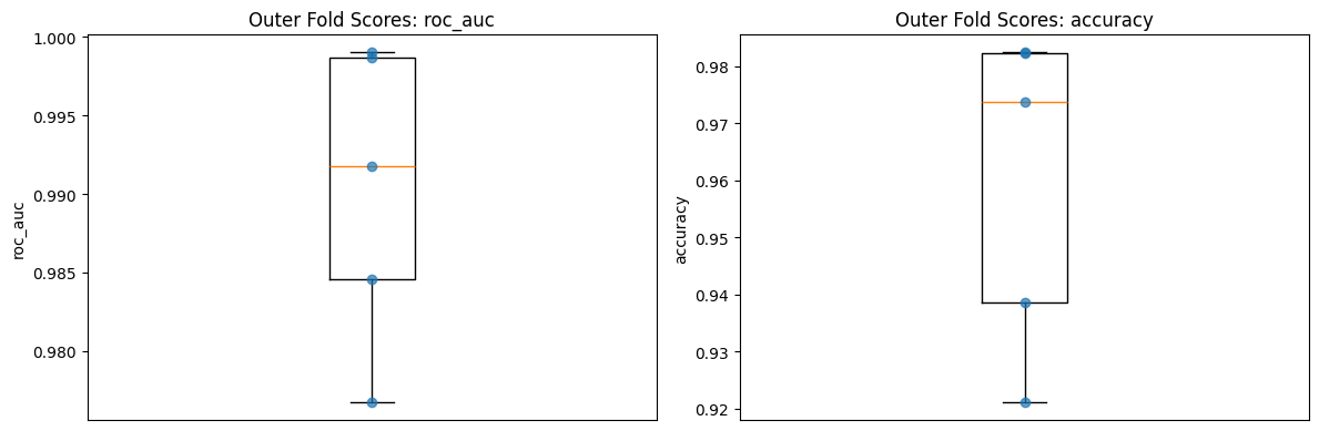
[9]:
fig, axes = plt.subplots(1, 2, figsize=(12, 4))
plot_outer_scores(results, "roc_auc", ax=axes[0])
plot_outer_scores(results, "accuracy", ax=axes[1])
plt.tight_layout()
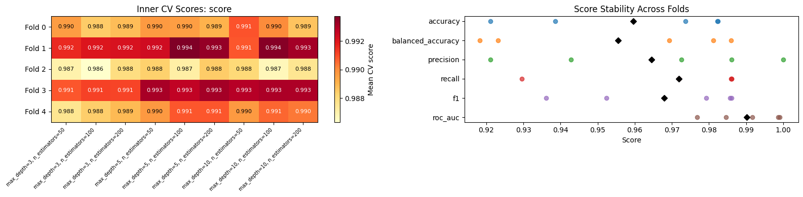
[10]:
fig, axes = plt.subplots(1, 2, figsize=(16, 4))
plot_inner_cv_heatmap(results, ax=axes[0])
plot_score_stability(results, ax=axes[1])
plt.tight_layout()
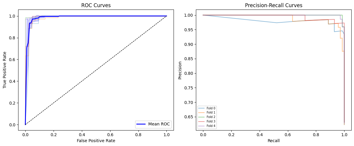
[11]:
fig, axes = plt.subplots(1, 2, figsize=(12, 5))
plot_roc_curves(results, ax=axes[0])
plot_precision_recall_curves(results, ax=axes[1])
plt.tight_layout()
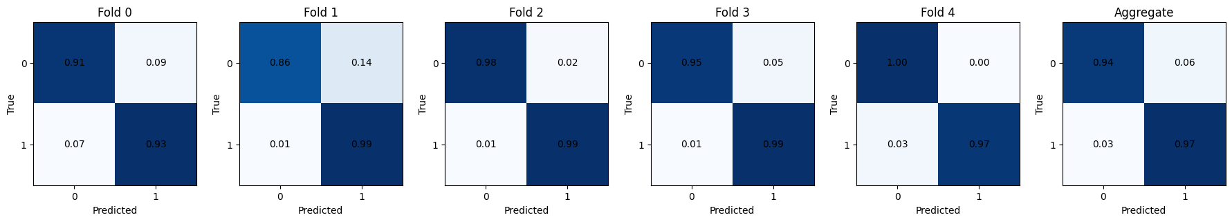
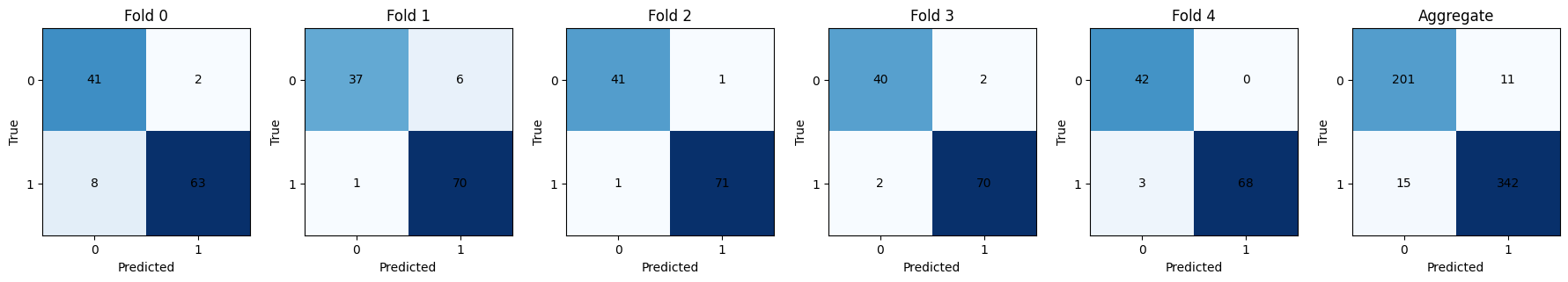
[12]:
plot_confusion_matrices(results, normalize="true")
[12]:
<Axes: title={'center': 'Fold 0'}, xlabel='Predicted', ylabel='True'>
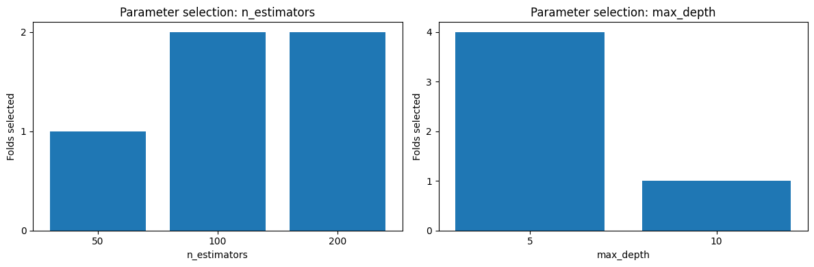
[13]:
# Which hyperparameters were selected across folds?
fig, axes = plt.subplots(1, 2, figsize=(12, 4))
plot_param_selection(results, "n_estimators", ax=axes[0])
plot_param_selection(results, "max_depth", ax=axes[1])
plt.tight_layout()
4. Adding Probability Calibration#
Many classifiers produce poorly calibrated probabilities - a predicted probability of 0.8 doesn’t mean the event occurs 80% of the time. nestkit supports four post-hoc calibration methods:
"sigmoid"- Platt scaling (logistic regression on raw probabilities)"isotonic"- Isotonic regression (non-parametric)"beta"- Beta calibration"venn-abers"- Venn-ABERS prediction
Calibration is performed using out-of-fold (OOF) predictions from the inner CV to avoid data leakage.
[14]:
ncv_cal = NestedCVClassifier(
    estimator=RandomForestClassifier(random_state=42),
    param_grid={"n_estimators": [50, 100, 200], "max_depth": [3, 5, 10]},
    outer_cv=5,
    inner_cv=3,
    scoring="roc_auc",
    calibration_method="isotonic",
    random_state=42,
)
ncv_cal.fit(X, y)
results_cal = ncv_cal.results_
[15]:
print(f"Has calibration: {results_cal.has_calibration}")
print("\nCalibration summary (per-fold ECE, Brier scores):")
display(results_cal.calibration_summary_)
print("\nCalibration improvement (delta = raw - calibrated, positive = improvement):")
display(results_cal.calibration_improvement_)
Has calibration: True

Calibration summary (per-fold ECE, Brier scores):
| fold_idx | ece_raw | ece_calibrated | mce_raw | mce_calibrated | brier_raw | brier_calibrated | |
|---|---|---|---|---|---|---|---|
| 0 | 0 | 0.042456 | 0.019309 | 0.152000 | 0.175926 | 0.043832 | 0.045787 |
| 1 | 1 | 0.040486 | 0.052332 | 0.205041 | 0.344236 | 0.045089 | 0.054155 |
| 2 | 2 | 0.040498 | 0.016296 | 0.142264 | 0.080141 | 0.019292 | 0.015467 |
| 3 | 3 | 0.031108 | 0.007254 | 0.139114 | 0.011426 | 0.030284 | 0.028567 |
| 4 | 4 | 0.042710 | 0.019833 | 0.201191 | 0.244089 | 0.020169 | 0.016963 |
Calibration improvement (delta = raw - calibrated, positive = improvement):
| fold_idx | delta_ece | delta_brier | |
|---|---|---|---|
| 0 | 0.0 | 0.023147 | -0.001955 |
| 1 | 1.0 | -0.011845 | -0.009066 |
| 2 | 2.0 | 0.024202 | 0.003825 |
| 3 | 3.0 | 0.023854 | 0.001717 |
| 4 | 4.0 | 0.022878 | 0.003206 |
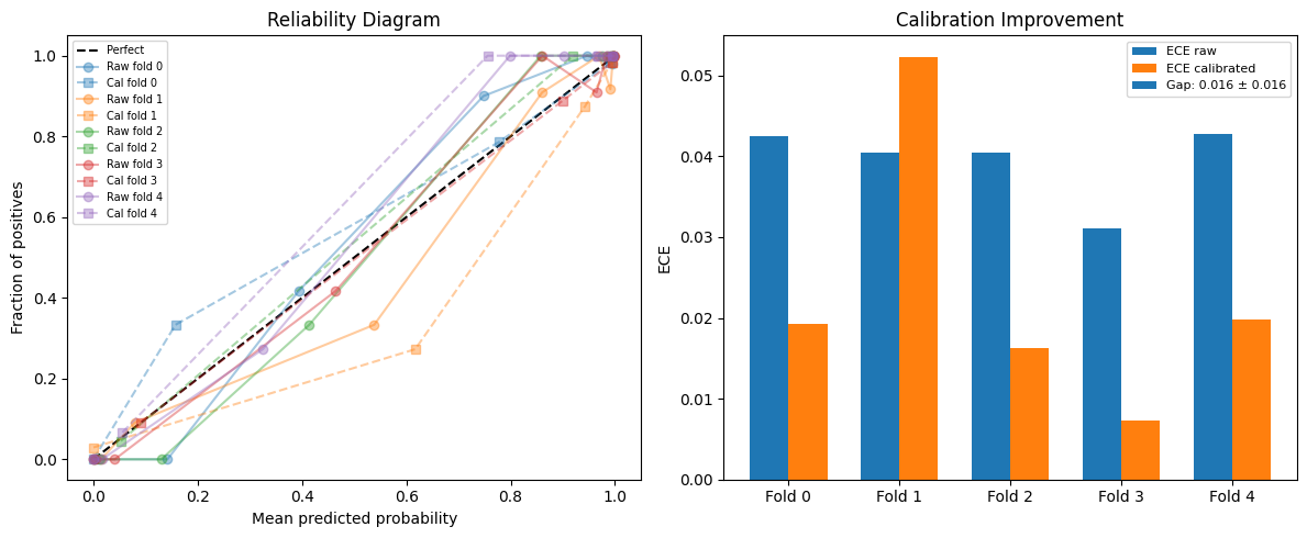
[16]:
fig, axes = plt.subplots(1, 2, figsize=(12, 5))
plot_calibration_curves(results_cal, ax=axes[0])
plot_calibration_improvement(results_cal, ax=axes[1])
plt.tight_layout()
5. Adding Threshold Optimization#
The default decision threshold of 0.5 is often suboptimal. nestkit can select an optimal threshold using several criteria:
"youden"- Maximizes Youden’s J statistic (sensitivity + specificity - 1)"f_beta"- Maximizes F-beta score"cost"- Minimizes expected cost given a cost matrix"balanced_accuracy"- Maximizes balanced accuracy"precision_at_recall"- Maximizes precision subject to a minimum recall
Two strategies are available:
"pooled"- A single threshold selected from all OOF predictions"fold_specific"- A separate threshold per outer fold
[17]:
ncv_thr = NestedCVClassifier(
    estimator=RandomForestClassifier(random_state=42),
    param_grid={"n_estimators": [50, 100, 200], "max_depth": [3, 5, 10]},
    outer_cv=5,
    inner_cv=3,
    scoring="roc_auc",
    calibration_method="isotonic",
    threshold_strategy="pooled",
    threshold_criterion="youden",
    random_state=42,
)
ncv_thr.fit(X, y)
results_thr = ncv_thr.results_
[18]:
print(f"Threshold optimization: {results_thr.has_threshold_optimization}")
print(f"\nThresholds per fold: {results_thr.thresholds_per_fold_}")
print(f"\nThreshold stability: {results_thr.threshold_stability_}")
Threshold optimization: True

Thresholds per fold: [0.6009697  0.5009899  0.44456566 0.41684848 0.5009899 ]

Threshold stability: {'mean': 0.4928727272727273, 'std': 0.07058680883762491, 'cv': 0.14321508359382815, 'range': 0.18412121212121219}
[19]:
# Side-by-side comparison: default (0.5) vs optimized threshold
results_thr.threshold_comparison()
[19]:
| metric | mean_default | std_default | mean_optimized | std_optimized | |
|---|---|---|---|---|---|
| 0 | accuracy | 0.959603 | 0.020154 | 0.954339 | 0.028655 |
| 1 | balanced_accuracy | 0.953631 | 0.024760 | 0.953184 | 0.029577 |
| 2 | precision | 0.959211 | 0.026155 | 0.969723 | 0.029835 |
| 3 | recall | 0.977582 | 0.012588 | 0.957864 | 0.041130 |
| 4 | f1 | 0.968157 | 0.015799 | 0.963120 | 0.024000 |
| 5 | roc_auc | 0.986868 | 0.012304 | 0.986868 | 0.012304 |
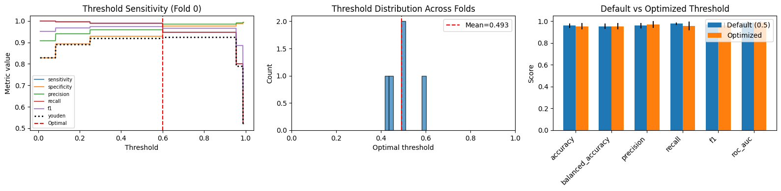
[20]:
fig, axes = plt.subplots(1, 3, figsize=(16, 4))
plot_threshold_sensitivity(results_thr, fold_idx=0, ax=axes[0])
plot_threshold_distribution(results_thr, bins=10, full_range=True, ax=axes[1])
plot_threshold_comparison(results_thr, ax=axes[2])
plt.tight_layout()
[21]:
# Confusion matrices with optimized threshold
plot_confusion_matrices(results_thr, threshold="optimized")
[21]:
<Axes: title={'center': 'Fold 0'}, xlabel='Predicted', ylabel='True'>
6. Regression with NestedCVRegressor#
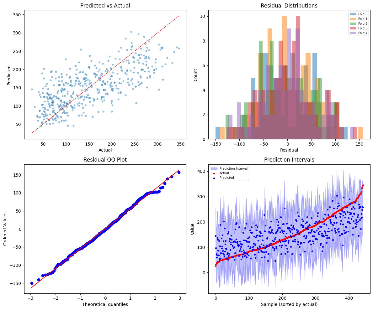
nestkit also supports regression tasks. NestedCVRegressor provides the same nested CV framework with optional residual-based prediction intervals - uncertainty estimates derived from the distribution of inner CV residuals.
[22]:
X_reg, y_reg = load_diabetes(return_X_y=True)
print(f"Shape: {X_reg.shape}, target range: [{y_reg.min():.0f}, {y_reg.max():.0f}]")
Shape: (442, 10), target range: [25, 346]
[23]:
ncv_reg = NestedCVRegressor(
    estimator=Ridge(),
    param_grid={"alpha": [0.01, 0.1, 1.0, 10.0, 100.0]},
    outer_cv=5,
    inner_cv=3,
    prediction_intervals=True,
    random_state=42,
)
ncv_reg.fit(X_reg, y_reg)
results_reg = ncv_reg.results_
[24]:
print("Summary:")
display(results_reg.summary_default_)
print(f"\nResidual stats: {results_reg.residual_stats_}")
print(f"\nPrediction interval coverage: {results_reg.prediction_interval_coverage_}")
Summary:
| metric | mean | std | ci_lower | ci_upper | median | iqr | |
|---|---|---|---|---|---|---|---|
| 0 | mse | 2997.691750 | 143.786002 | 2729.890897 | 3265.492603 | 3001.755668 | 104.319504 |
| 1 | rmse | 54.738582 | 1.313080 | 52.292975 | 57.184189 | 54.788280 | 0.953475 |
| 2 | mae | 44.294273 | 2.179699 | 40.234593 | 48.353953 | 43.292787 | 2.100991 |
| 3 | r2 | 0.481443 | 0.054231 | 0.380438 | 0.582447 | 0.489191 | 0.092220 |
| 4 | mape | 0.394409 | 0.032817 | 0.333288 | 0.455530 | 0.391332 | 0.044576 |
Residual stats: {'mean': 0.37101618492788285, 'std': 54.80893629831313, 'median': -2.1691076714726307, 'skewness': 0.05688818733292645, 'kurtosis': -0.2869504563698184}

Prediction interval coverage: {'mean': 0.9547242083758938, 'per_fold': [0.9550561797752809, 0.9662921348314607, 0.9659090909090909, 0.9204545454545454, 0.9659090909090909]}
[25]:
fig, axes = plt.subplots(2, 2, figsize=(12, 10))
plot_predicted_vs_actual(results_reg, ax=axes[0, 0])
plot_residuals(results_reg, ax=axes[0, 1])
plot_residual_qq(results_reg, ax=axes[1, 0])
plot_prediction_intervals(results_reg, ax=axes[1, 1])
plt.tight_layout()
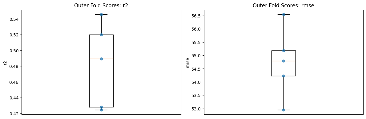
[26]:
fig, axes = plt.subplots(1, 2, figsize=(12, 4))
plot_outer_scores(results_reg, "r2", ax=axes[0])
plot_outer_scores(results_reg, "rmse", ax=axes[1])
plt.tight_layout()
Next Steps#
This notebook covered the core nestkit workflow. For advanced topics, see 02 - Advanced Workflows:
Multi-model statistical comparison with
NestedCVComparatorFeature importance aggregation with
FeatureImportanceAggregatorHyperparameter stability diagnostics
Callbacks and persistence