Advanced Workflows with nestkit#
This notebook covers nestkit’s advanced analysis tools. It assumes familiarity with the basics covered in 01 - Basic Usage.
What you’ll learn#
Multi-model statistical comparison with
NestedCVComparatorFeature importance aggregation with
FeatureImportanceAggregatorHyperparameter stability diagnostics
Callbacks: progress, logging, checkpointing
Prerequisites#
pip install nestkit[full]
[1]:
import logging
import os
import tempfile
import time
import warnings

import matplotlib.pyplot as plt
from sklearn.datasets import load_breast_cancer, load_diabetes
from sklearn.ensemble import GradientBoostingClassifier, RandomForestClassifier
from sklearn.linear_model import LogisticRegression

from nestkit import NestedCVClassifier
from nestkit.callbacks import CheckpointCallback, LoggingCallback, ProgressCallback
from nestkit.comparison import NestedCVComparator
from nestkit.diagnostics import HyperparameterStability
from nestkit.importance import FeatureImportanceAggregator
from nestkit.plotting import (
    plot_bayesian_posterior,
    plot_comparison,
    plot_critical_difference,
    plot_importance,
    plot_rank_stability_features,
    plot_score_differences,
    plot_selection_frequency,
)

warnings.filterwarnings("ignore")

%matplotlib inline
plt.rcParams["figure.dpi"] = 100
0. Data Setup#
We reuse the same datasets from notebook 01 to maintain continuity. For multi-model comparison we need all models evaluated on identical outer folds, so we fix outer_cv=5, inner_cv=3, and random_state=42 throughout.
[2]:
X_clf, y_clf = load_breast_cancer(return_X_y=True)
feature_names_clf = list(load_breast_cancer().feature_names)

X_reg, y_reg = load_diabetes(return_X_y=True)
feature_names_reg = list(load_diabetes().feature_names)

print(f"Classification: {X_clf.shape}, Regression: {X_reg.shape}")
Classification: (569, 30), Regression: (442, 10)
1. Multi-Model Statistical Comparison#
A common question is: “Is model A really better than model B?” Simply comparing mean scores is unreliable because outer-fold scores are correlated (overlapping training sets). NestedCVComparator provides three principled approaches:
Nadeau-Bengio corrected paired t-test - frequentist test that corrects for the non-independence of CV folds
Bayesian correlated t-test with ROPE - gives posterior probabilities that model A is better, practically equivalent, or worse
Critical difference diagram - visual ranking of 3+ models (Demsar, 2006)
1.1 Fitting multiple models on identical folds#
[3]:
# All models share identical outer_cv, inner_cv, random_state
common = dict(outer_cv=5, inner_cv=3, scoring="roc_auc", random_state=42)

# Model 1: Random Forest
ncv_rf = NestedCVClassifier(
    estimator=RandomForestClassifier(random_state=42),
    param_grid={"n_estimators": [50, 100, 200], "max_depth": [3, 5, 10]},
    **common,
)
ncv_rf.fit(X_clf, y_clf)

# Model 2: Logistic Regression
ncv_lr = NestedCVClassifier(
    estimator=LogisticRegression(max_iter=5000, random_state=42),
    param_grid={"C": [0.01, 0.1, 1.0, 10.0], "penalty": ["l1", "l2"], "solver": ["saga"]},
    **common,
)
ncv_lr.fit(X_clf, y_clf)

# Model 3: Gradient Boosting
ncv_gb = NestedCVClassifier(
    estimator=GradientBoostingClassifier(random_state=42),
    param_grid={"n_estimators": [50, 100], "max_depth": [2, 3, 5], "learning_rate": [0.05, 0.1]},
    **common,
)
ncv_gb.fit(X_clf, y_clf)

print("All models fitted.")
All models fitted.
1.2 Building the comparator#
Register each model’s results under a human-readable name. NestedCVComparator validates that all models share identical outer-fold indices.
[4]:
comparator = NestedCVComparator()
comparator.add("Random Forest", ncv_rf.results_)
comparator.add("Logistic Regression", ncv_lr.results_)
comparator.add("Gradient Boosting", ncv_gb.results_)

display(comparator.summary("roc_auc"))
| model | mean | std | median | ci_lower | ci_upper | min | max | iqr | |
|---|---|---|---|---|---|---|---|---|---|
| 0 | Random Forest | 0.990150 | 0.009537 | 0.991733 | 0.972387 | 1.007913 | 0.976744 | 0.999008 | 0.014053 |
| 1 | Logistic Regression | 0.969716 | 0.011034 | 0.970899 | 0.949166 | 0.990267 | 0.956436 | 0.985260 | 0.011104 |
| 2 | Gradient Boosting | 0.991837 | 0.006119 | 0.990829 | 0.980441 | 1.003233 | 0.985450 | 0.998347 | 0.011417 |
[5]:
# Rank models by mean ROC AUC
display(comparator.rank_models("roc_auc"))
| model | mean | std | median | ci_lower | ci_upper | min | max | iqr | rank | |
|---|---|---|---|---|---|---|---|---|---|---|
| 0 | Gradient Boosting | 0.991837 | 0.006119 | 0.990829 | 0.980441 | 1.003233 | 0.985450 | 0.998347 | 0.011417 | 1 |
| 1 | Random Forest | 0.990150 | 0.009537 | 0.991733 | 0.972387 | 1.007913 | 0.976744 | 0.999008 | 0.014053 | 2 |
| 2 | Logistic Regression | 0.969716 | 0.011034 | 0.970899 | 0.949166 | 0.990267 | 0.956436 | 0.985260 | 0.011104 | 3 |
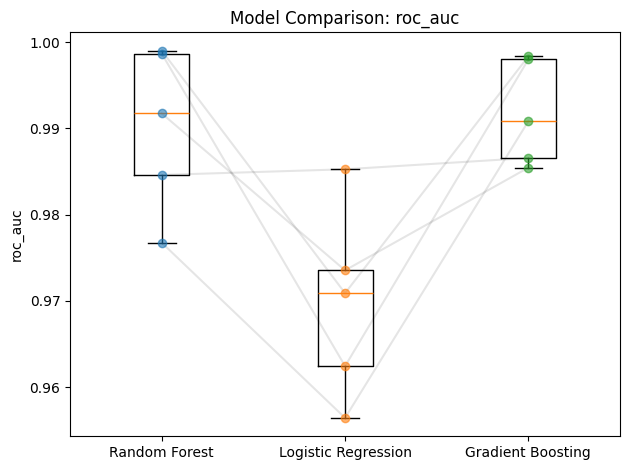
1.3 Visual comparison#
plot_comparison draws paired box-and-strip plots with lines connecting the same fold across models - making it easy to spot whether one model consistently wins.
[6]:
plot_comparison(comparator, "roc_auc", line_alpha=0.1)
plt.tight_layout()
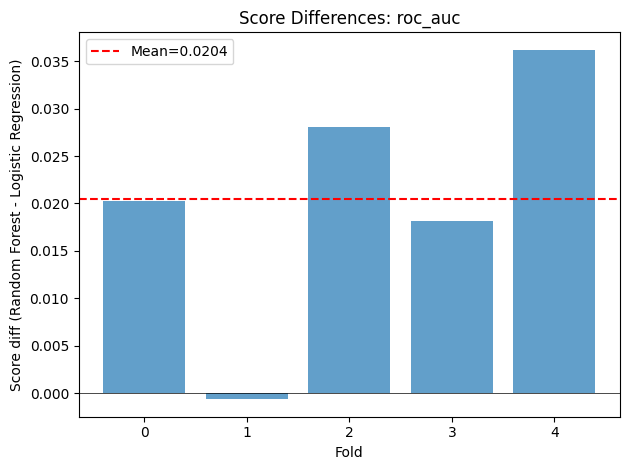
1.4 Nadeau-Bengio corrected paired t-test#
Standard paired t-tests underestimate the variance of CV scores because training sets overlap. The Nadeau-Bengio correction (2003) adjusts the variance estimate by accounting for the ratio of test-set size to training-set size.
[7]:
# Single pairwise test
result = comparator.corrected_paired_ttest("roc_auc", "Random Forest", "Logistic Regression")
print("RF vs LR (Nadeau-Bengio corrected):")
for k, v in result.items():
    print(f"  {k}: {v}")
RF vs LR (Nadeau-Bengio corrected):
  t_statistic: 2.212985001740397
  p_value: 0.0913221564679729
  mean_difference: 0.020433280128661656
  corrected_std: 0.009233356806572095
  ci_lower: -0.005202628181490216
  ci_upper: 0.046069188438813524
  n_folds: 5
  significant_at_005: False
  significant_at_001: False
[8]:
# All pairwise tests with Holm-Bonferroni correction for multiple comparisons
display(comparator.pairwise_corrected_ttest("roc_auc"))
| model_a | model_b | t_statistic | p_value | mean_difference | corrected_std | ci_lower | ci_upper | n_folds | significant_at_005 | significant_at_001 | p_value_corrected | |
|---|---|---|---|---|---|---|---|---|---|---|---|---|
| 0 | Random Forest | Logistic Regression | 2.212985 | 0.091322 | 0.020433 | 0.009233 | -0.005203 | 0.046069 | 5 | False | False | 0.273966 |
| 1 | Random Forest | Gradient Boosting | -0.332813 | 0.755988 | -0.001687 | 0.005069 | -0.015760 | 0.012386 | 5 | False | False | 0.755988 |
| 2 | Logistic Regression | Gradient Boosting | -2.202411 | 0.092404 | -0.022120 | 0.010044 | -0.050006 | 0.005765 | 5 | False | False | 0.273966 |
[9]:
plot_score_differences(comparator, "roc_auc", "Random Forest", "Logistic Regression")
plt.tight_layout()
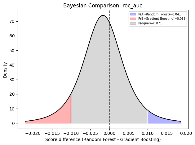
1.5 Bayesian correlated t-test with ROPE#
The Bayesian test (Benavoli et al., 2017) partitions the posterior probability mass into three regions:
P(A better) - model A’s mean score exceeds model B’s by more than the ROPE
P(equivalent) - the difference lies within the Region of Practical Equivalence
P(B better) - model B’s mean score exceeds model A’s by more than the ROPE
This avoids the binary “significant / not significant” dichotomy and quantifies practical equivalence.
[10]:
bayes = comparator.bayesian_comparison("roc_auc", "Random Forest", "Gradient Boosting", rope=0.01)
print("Bayesian comparison (RF vs GB):")
for k, v in bayes.items():
    print(f"  {k}: {v:.4f}" if isinstance(v, float) else f"  {k}: {v}")
Bayesian comparison (RF vs GB):
  p_a_better: 0.0412
  p_equivalent: 0.8706
  p_b_better: 0.0882
  rope: 0.0100
  mean_difference: -0.0017
  hdi_lower: -0.0158
  hdi_upper: 0.0124
[11]:
plot_bayesian_posterior(comparator, "roc_auc", "Random Forest", "Gradient Boosting", rope=0.01)
plt.tight_layout()
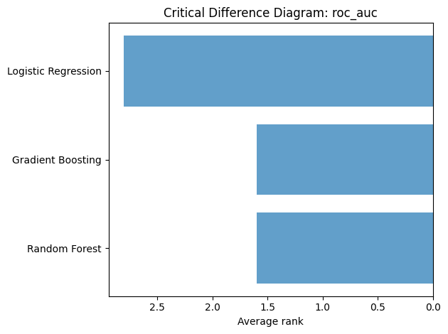
1.6 Critical difference diagram#
When comparing three or more models, a critical difference diagram (Demsar, 2006) ranks models by their average rank across folds and groups models that are not significantly different.
[12]:
plot_critical_difference(comparator, "roc_auc")
plt.tight_layout()
2. Feature Importance Analysis#
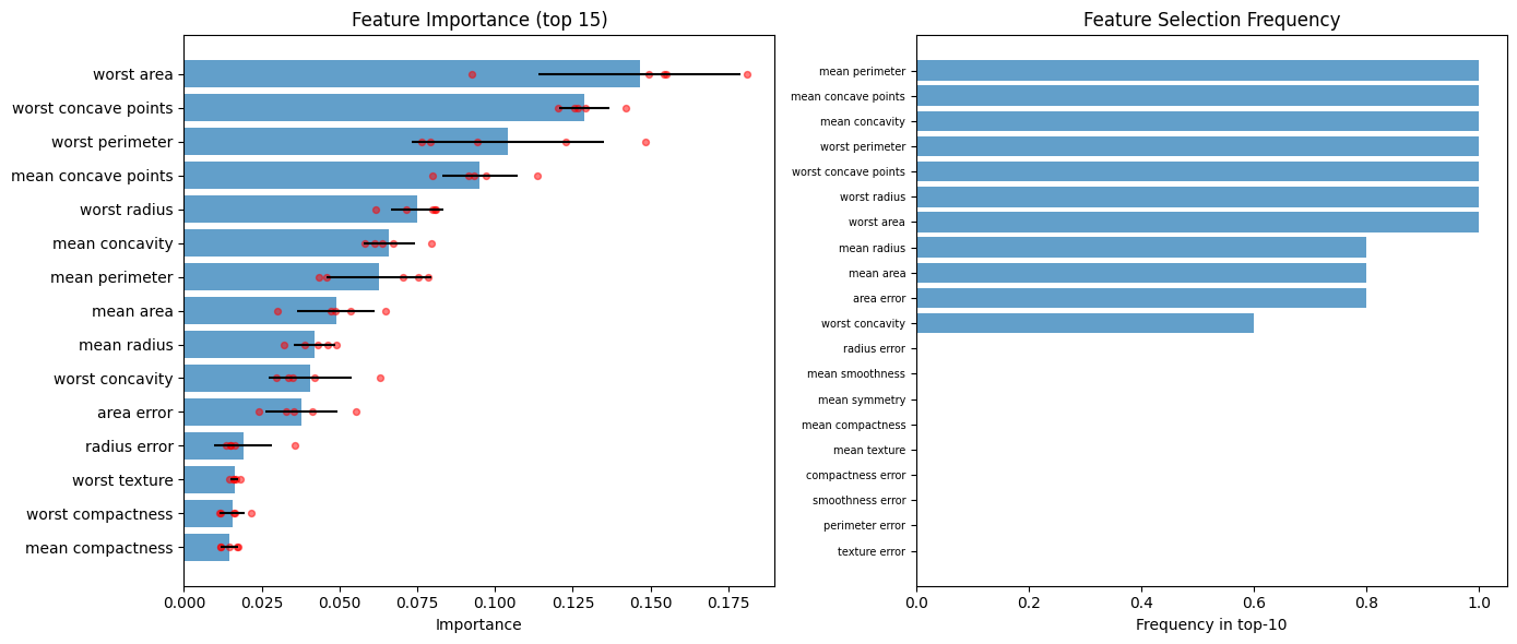
Feature importances from a single train/test split can be noisy and misleading. FeatureImportanceAggregator extracts importances from each outer-fold estimator, aggregates them, and assesses their stability - how consistently the same features are ranked important across folds.
Key outputs:
Summary table - mean, std, CV, and rank statistics per feature
Nogueira stability index - measures agreement of top-k feature sets across folds (1 = perfect, 0 = random)
Consensus features - features that reliably appear in the top-k across folds
[13]:
agg = FeatureImportanceAggregator(
    ncv_rf.results_,
    method="model",
    feature_names=feature_names_clf,
)
agg.compute()

print("Top 10 features by mean importance:")
display(agg.summary_.head(10))
Top 10 features by mean importance:
| feature | mean_importance | std_importance | median_importance | min_importance | max_importance | cv_importance | mean_rank | std_rank | |
|---|---|---|---|---|---|---|---|---|---|
| 0 | worst area | 0.146445 | 0.032512 | 0.154264 | 0.092618 | 0.180883 | 0.222011 | 1.6 | 1.341641 |
| 1 | worst concave points | 0.128764 | 0.008015 | 0.126759 | 0.120410 | 0.141930 | 0.062244 | 2.2 | 0.836660 |
| 2 | worst perimeter | 0.104169 | 0.030896 | 0.094333 | 0.076230 | 0.148497 | 0.296590 | 3.6 | 1.816590 |
| 3 | mean concave points | 0.095041 | 0.012074 | 0.093302 | 0.080057 | 0.113452 | 0.127036 | 3.4 | 0.894427 |
| 4 | worst radius | 0.074889 | 0.008408 | 0.079846 | 0.061508 | 0.080985 | 0.112277 | 4.8 | 1.303840 |
| 5 | mean concavity | 0.066027 | 0.008330 | 0.063741 | 0.057992 | 0.079635 | 0.126155 | 6.4 | 0.894427 |
| 6 | mean perimeter | 0.062685 | 0.016754 | 0.070298 | 0.043445 | 0.078647 | 0.267271 | 7.0 | 1.581139 |
| 7 | mean area | 0.048882 | 0.012535 | 0.048680 | 0.030149 | 0.064769 | 0.256436 | 8.8 | 1.303840 |
| 8 | mean radius | 0.041921 | 0.006607 | 0.043092 | 0.032296 | 0.049127 | 0.157613 | 9.4 | 1.816590 |
| 9 | worst concavity | 0.040636 | 0.013206 | 0.034822 | 0.029775 | 0.062906 | 0.324974 | 9.4 | 2.509980 |
[14]:
fig, axes = plt.subplots(1, 2, figsize=(14, 6))
plot_importance(agg, top_k=15, ax=axes[0])
plot_selection_frequency(agg, top_k=10, ax=axes[1])
plt.tight_layout()
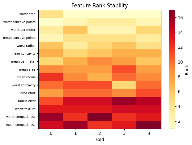
2.1 Nogueira stability index#
The Nogueira et al. (2018) stability index measures how consistently the same features appear in the top-k set across folds, corrected for chance agreement. Values near 1 indicate high stability; values near 0 indicate that top features vary across folds.
[15]:
for k in [5, 10, 15]:
    idx = agg.stability_index(top_k=k)
    print(f"Stability index (top-{k}): {idx:.4f}")
Stability index (top-5): 0.7360
Stability index (top-10): 0.8650
Stability index (top-15): 0.7867
[16]:
plot_rank_stability_features(agg, top_k=15)
plt.tight_layout()
2.2 Consensus features#
Two strategies for identifying reliably important features:
"top_k"- the top-k features by mean importance"frequency"- features appearing in the top-k in at least a given fraction of folds (more conservative)
[17]:
# Top-10 by mean importance
top10 = agg.consensus_features(criterion="top_k", top_k=10)
print(f"Top-10 by mean importance:\n  {top10}\n")

# Features in top-10 in at least 80% of folds
consensus = agg.consensus_features(criterion="frequency", top_k=10, min_frequency=0.8)
print(f"Consensus features (top-10, >=80% folds):\n  {consensus}")
Top-10 by mean importance:
  [np.str_('worst area'), np.str_('worst concave points'), np.str_('worst perimeter'), np.str_('mean concave points'), np.str_('worst radius'), np.str_('mean concavity'), np.str_('mean perimeter'), np.str_('mean area'), np.str_('mean radius'), np.str_('worst concavity')]

Consensus features (top-10, >=80% folds):
  [np.str_('mean radius'), np.str_('mean perimeter'), np.str_('mean area'), np.str_('mean concavity'), np.str_('mean concave points'), np.str_('area error'), np.str_('worst radius'), np.str_('worst perimeter'), np.str_('worst area'), np.str_('worst concave points')]
[18]:
# Pairwise Spearman rank correlation between folds
print("Pairwise Spearman rank correlation:")
display(agg.pairwise_rank_correlation())
Pairwise Spearman rank correlation:
| fold_i | fold_j | spearman_r | p_value | |
|---|---|---|---|---|
| 0 | 0 | 1 | 0.933704 | 5.157534e-14 |
| 1 | 0 | 2 | 0.920801 | 5.735790e-13 |
| 2 | 0 | 3 | 0.954171 | 3.333087e-16 |
| 3 | 0 | 4 | 0.926140 | 2.232463e-13 |
| 4 | 1 | 2 | 0.939488 | 1.489555e-14 |
| 5 | 1 | 3 | 0.948832 | 1.508414e-15 |
| 6 | 1 | 4 | 0.964850 | 8.680629e-18 |
| 7 | 2 | 3 | 0.948387 | 1.698100e-15 |
| 8 | 2 | 4 | 0.953726 | 3.805360e-16 |
| 9 | 3 | 4 | 0.952836 | 4.941027e-16 |
3. Hyperparameter Stability Diagnostics#
If the inner CV selects different hyperparameters in different outer folds, the model may be sensitive to the training data composition. HyperparameterStability diagnoses this by computing:
Mode and agreement rate - how often each parameter’s most-common value was selected
Entropy - low entropy means consistent selection
Pairwise Jaccard similarity - how similar the full configuration sets are across folds
[19]:
hs_rf = HyperparameterStability(ncv_rf.results_.best_params_per_fold_)

print("RF hyperparameter stability summary:")
display(hs_rf.summary())
RF hyperparameter stability summary:
| param | mode | nunique | entropy | agreement_rate | cv | |
|---|---|---|---|---|---|---|
| 0 | max_depth | 5 | 2 | 0.721928 | 0.8 | 0.372678 |
| 1 | n_estimators | 100 | 3 | 1.521928 | 0.4 | 0.516016 |
[20]:
# Which parameters are stable (>=80% agreement)?
print("Stable parameters:", hs_rf.is_stable(threshold=0.8))

print("\nPairwise Jaccard similarity between fold configurations:")
display(hs_rf.pairwise_jaccard())
Stable parameters: {'max_depth': True, 'n_estimators': False}

Pairwise Jaccard similarity between fold configurations:
| fold_i | fold_j | jaccard | |
|---|---|---|---|
| 0 | 0 | 1 | 0.000000 |
| 1 | 0 | 2 | 0.000000 |
| 2 | 0 | 3 | 0.000000 |
| 3 | 0 | 4 | 0.000000 |
| 4 | 1 | 2 | 0.333333 |
| 5 | 1 | 3 | 0.333333 |
| 6 | 1 | 4 | 1.000000 |
| 7 | 2 | 3 | 1.000000 |
| 8 | 2 | 4 | 0.333333 |
| 9 | 3 | 4 | 0.333333 |
[21]:
# Compare stability across all three models
for name, ncv in [("RF", ncv_rf), ("LR", ncv_lr), ("GB", ncv_gb)]:
    hs = HyperparameterStability(ncv.results_.best_params_per_fold_)
    summary = hs.summary()
    mean_agreement = summary["agreement_rate"].mean()
    mean_entropy = summary["entropy"].mean()
    print(f"{name}: mean agreement={mean_agreement:.2f}, mean entropy={mean_entropy:.2f}")
RF: mean agreement=0.60, mean entropy=1.12
LR: mean agreement=0.80, mean entropy=0.56
GB: mean agreement=0.80, mean entropy=0.56
4. Conformal Prediction#
nestkit supports CV+ Mondrian conformal prediction for both classification and regression.
Classifier: per-class conformal quantile thresholds produce prediction sets with formal coverage guarantees
Regressor: Mondrian binning by predicted value yields conditional prediction intervals that are tighter in easy-to-predict regions
Conformal prediction runs after calibration and threshold optimization, using calibrated OOF probabilities when available.
4.1 Classifier conformal prediction sets#
Enable conformal prediction with conformal_prediction=True. The conformal_alpha parameter controls the target miscoverage rate (default 0.1 = 90% target coverage).
[22]:
ncv_conformal = NestedCVClassifier(
    estimator=RandomForestClassifier(random_state=42),
    param_grid={"n_estimators": [50, 100], "max_depth": [3, 5]},
    outer_cv=5,
    inner_cv=3,
    scoring="roc_auc",
    random_state=42,
    conformal_prediction=True,
    conformal_alpha=0.1,
)
ncv_conformal.fit(X_clf, y_clf)

print("Conformal prediction enabled:", ncv_conformal.results_.has_conformal)
print(f"Mean coverage: {ncv_conformal.results_.conformal_coverage_['mean']:.3f}")
print(f"Mean set size: {ncv_conformal.results_.conformal_set_size_stats_['mean']:.3f}")
Conformal prediction enabled: True
Mean coverage: 0.907
Mean set size: 0.924
[23]:
# Per-fold conformal report
display(ncv_conformal.results_.conformal_report())
| fold_idx | coverage | mean_set_size | frac_singleton | frac_empty | |
|---|---|---|---|---|---|
| 0 | 0 | 0.877193 | 0.912281 | 0.912281 | 0.087719 |
| 1 | 1 | 0.868421 | 0.894737 | 0.894737 | 0.105263 |
| 2 | 2 | 0.964912 | 0.973684 | 0.973684 | 0.026316 |
| 3 | 3 | 0.894737 | 0.903509 | 0.903509 | 0.096491 |
| 4 | 4 | 0.929204 | 0.938053 | 0.938053 | 0.061947 |
[24]:
# Predictions DataFrame now includes conformal_set_size and conformal_in_set
display(
    ncv_conformal.results_.predictions_[
        ["y_true", "y_pred_default", "conformal_set_size", "conformal_in_set"]
    ].head(10)
)
| y_true | y_pred_default | conformal_set_size | conformal_in_set | |
|---|---|---|---|---|
| 0 | 0 | 0 | 1 | True |
| 1 | 0 | 0 | 1 | True |
| 2 | 0 | 0 | 1 | True |
| 3 | 0 | 0 | 1 | True |
| 4 | 0 | 0 | 1 | True |
| 5 | 0 | 0 | 1 | True |
| 6 | 0 | 0 | 1 | True |
| 7 | 0 | 0 | 1 | True |
| 8 | 0 | 0 | 1 | True |
| 9 | 0 | 0 | 1 | True |
4.2 Combining calibration + threshold + conformal#
All three post-hoc features compose naturally. When calibration is enabled, conformal thresholds are computed from calibrated probabilities.
[25]:
ncv_full = NestedCVClassifier(
    estimator=RandomForestClassifier(random_state=42),
    param_grid={"n_estimators": [50, 100], "max_depth": [3, 5]},
    outer_cv=5,
    inner_cv=3,
    scoring="roc_auc",
    random_state=42,
    calibration_method="isotonic",
    threshold_strategy="pooled",
    conformal_prediction=True,
    conformal_alpha=0.1,
)
ncv_full.fit(X_clf, y_clf)

r = ncv_full.results_
print(
    f"Calibration: {r.has_calibration}, Threshold: {r.has_threshold_optimization}, Conformal: {r.has_conformal}"
)
print(f"Mean conformal coverage: {r.conformal_coverage_['mean']:.3f}")
print(f"q-hat stability (std per class): {r.conformal_qhat_stability_['std_per_class']}")
Calibration: True, Threshold: True, Conformal: True
Mean conformal coverage: 0.928
q-hat stability (std per class): [0.14066273709105082, 0.07630643735352548]
4.3 Regressor: Mondrian prediction intervals#
For regression, mondrian_bins enables Mondrian-style conditional prediction intervals. OOF predictions are grouped into equal-frequency bins, and per-bin residual quantiles give tighter intervals in easy-to-predict regions.
[26]:
from sklearn.ensemble import RandomForestRegressor

from nestkit import NestedCVRegressor

ncv_reg_mondrian = NestedCVRegressor(
    estimator=RandomForestRegressor(random_state=42),
    param_grid={"n_estimators": [50, 100], "max_depth": [5, 10]},
    outer_cv=5,
    inner_cv=3,
    random_state=42,
    prediction_intervals=True,
    confidence_level=0.90,
    mondrian_bins=3,
)
ncv_reg_mondrian.fit(X_reg, y_reg)

r_reg = ncv_reg_mondrian.results_
print(f"Overall coverage: {r_reg.prediction_interval_coverage_['mean']:.3f}")
print(f"Per-bin coverage: {r_reg.mondrian_coverage_per_bin_}")
Overall coverage: 0.909
Per-bin coverage: {0: 0.9054054054054054, 1: 0.9266666666666666, 2: 0.8958333333333334}
[27]:
# Predictions include per-sample bin assignments and intervals
display(
    ncv_reg_mondrian.results_.predictions_[
        ["y_true", "y_pred", "pi_lower", "pi_upper", "mondrian_bin"]
    ].head(10)
)
| y_true | y_pred | pi_lower | pi_upper | mondrian_bin | |
|---|---|---|---|---|---|
| 0 | 151.0 | 215.932084 | 106.851684 | 303.158261 | 2 |
| 1 | 75.0 | 85.428902 | 29.613270 | 188.323636 | 0 |
| 2 | 141.0 | 181.896152 | 72.815752 | 269.122328 | 2 |
| 3 | 206.0 | 157.863997 | 72.079456 | 294.932256 | 1 |
| 4 | 135.0 | 95.199586 | 39.383955 | 198.094321 | 0 |
| 5 | 97.0 | 102.992719 | 47.177088 | 205.887454 | 0 |
| 6 | 138.0 | 82.646132 | 26.830501 | 185.540867 | 0 |
| 7 | 63.0 | 142.896578 | 57.112037 | 279.964837 | 1 |
| 8 | 110.0 | 157.771662 | 71.987120 | 294.839921 | 1 |
| 9 | 310.0 | 174.042726 | 88.258184 | 311.110985 | 1 |
5. Callbacks#
nestkit supports a callback system that hooks into five lifecycle events:
on_outer_fold_start- before inner search beginson_inner_search_complete- after hyperparameter tuningon_post_processing_complete- after calibration / threshold optimizationon_outer_fold_complete- after outer fold evaluationon_nested_cv_complete- after all folds finish
Three built-in callbacks are provided:
Callback |
Purpose |
|---|---|
|
tqdm progress bar |
|
Structured log messages with timing |
|
Pickle fold results to disk after each fold |
Multiple callbacks can be combined by passing a list.
[28]:
# ProgressCallback  -  tqdm progress bar
ncv_progress = NestedCVClassifier(
    estimator=RandomForestClassifier(random_state=42),
    param_grid={"n_estimators": [50, 100], "max_depth": [3, 5]},
    outer_cv=5,
    inner_cv=3,
    scoring="roc_auc",
    random_state=42,
    callbacks=[ProgressCallback(n_outer_folds=5)],
)
ncv_progress.fit(X_clf, y_clf)
print("Done!")
Outer folds: 100%|██████████| 5/5 [00:03<00:00, 1.36it/s]
Done!
[29]:
# LoggingCallback  -  structured log messages
logging.basicConfig(level=logging.INFO, format="%(name)s | %(message)s", force=True)

ncv_logged = NestedCVClassifier(
    estimator=RandomForestClassifier(random_state=42),
    param_grid={"n_estimators": [50, 100], "max_depth": [3, 5]},
    outer_cv=5,
    inner_cv=3,
    scoring="roc_auc",
    random_state=42,
    callbacks=[LoggingCallback()],
)
ncv_logged.fit(X_clf, y_clf)
nestkit | Outer fold 0: starting
nestkit | Fold 0: started (train=455, test=114)
nestkit | Outer fold 0: inner search complete (0.6s), best_score=0.9897
nestkit | Fold 0: inner search complete, best_params={'max_depth': 5, 'n_estimators': 50}, best_score=0.9897
nestkit | Fold 0: post-processing complete
nestkit | Fold 0: complete (0.7s)
nestkit | Outer fold 0: complete
nestkit | Outer fold 1: starting
nestkit | Fold 1: started (train=455, test=114)
nestkit | Outer fold 1: inner search complete (0.7s), best_score=0.9937
nestkit | Fold 1: inner search complete, best_params={'max_depth': 5, 'n_estimators': 100}, best_score=0.9937
nestkit | Fold 1: post-processing complete
nestkit | Fold 1: complete (0.8s)
nestkit | Outer fold 1: complete
nestkit | Outer fold 2: starting
nestkit | Fold 2: started (train=455, test=114)
nestkit | Outer fold 2: inner search complete (0.7s), best_score=0.9884
nestkit | Fold 2: inner search complete, best_params={'max_depth': 5, 'n_estimators': 50}, best_score=0.9884
nestkit | Fold 2: post-processing complete
nestkit | Fold 2: complete (0.7s)
nestkit | Outer fold 2: complete
nestkit | Outer fold 3: starting
nestkit | Fold 3: started (train=455, test=114)
nestkit | Outer fold 3: inner search complete (0.7s), best_score=0.9931
nestkit | Fold 3: inner search complete, best_params={'max_depth': 5, 'n_estimators': 50}, best_score=0.9931
nestkit | Fold 3: post-processing complete
nestkit | Fold 3: complete (0.7s)
nestkit | Outer fold 3: complete
nestkit | Outer fold 4: starting
nestkit | Fold 4: started (train=456, test=113)
nestkit | Outer fold 4: inner search complete (0.7s), best_score=0.9908
nestkit | Fold 4: inner search complete, best_params={'max_depth': 5, 'n_estimators': 100}, best_score=0.9908
nestkit | Fold 4: post-processing complete
nestkit | Fold 4: complete (0.8s)
nestkit | Outer fold 4: complete
nestkit | Nested CV complete: 5 folds
[29]:
NestedCVClassifier(callbacks=[<nestkit.callbacks.LoggingCallback object at 0x7f01b058f370>],
                   estimator=RandomForestClassifier(random_state=42),
                   inner_cv=3,
                   param_grid={'max_depth': [3, 5], 'n_estimators': [50, 100]},
                   random_state=42, scoring='roc_auc')
In a Jupyter environment, please rerun this cell to show the HTML representation or trust the notebook. On GitHub, the HTML representation is unable to render, please try loading this page with nbviewer.org.
Parameters
| estimator | RandomForestC...ndom_state=42) | |
| param_grid | {'max_depth': [3, 5], 'n_estimators': [50, 100]} | |
| search_strategy | 'grid' | |
| outer_cv | 5 | |
| inner_cv | 3 | |
| scoring | 'roc_auc' | |
| refit | True | |
| return_train_score | False | |
| return_estimator | True | |
| error_score | 'raise' | |
| n_jobs_outer | None | |
| n_jobs_inner | None | |
| verbose | 0 | |
| random_state | 42 | |
| callbacks | [<nestkit.call...x7f01b058f370>] | |
| pre_dispatch | '2*n_jobs' | |
| calibration_method | None | |
| threshold_strategy | None | |
| threshold_criterion | 'youden' | |
| threshold_beta | 1.0 | |
| cost_matrix | None | |
| min_recall | None | |
| calibration_cv | None | |
| conformal_prediction | False | |
| conformal_alpha | 0.1 |
RandomForestClassifier(random_state=42)
Parameters
| n_estimators | 100 | |
| criterion | 'gini' | |
| max_depth | None | |
| min_samples_split | 2 | |
| min_samples_leaf | 1 | |
| min_weight_fraction_leaf | 0.0 | |
| max_features | 'sqrt' | |
| max_leaf_nodes | None | |
| min_impurity_decrease | 0.0 | |
| bootstrap | True | |
| oob_score | False | |
| n_jobs | None | |
| random_state | 42 | |
| verbose | 0 | |
| warm_start | False | |
| class_weight | None | |
| ccp_alpha | 0.0 | |
| max_samples | None | |
| monotonic_cst | None |
[30]:
# CheckpointCallback  -  saves fold results to disk
with tempfile.TemporaryDirectory() as tmpdir:
    checkpoint_dir = os.path.join(tmpdir, "ncv_checkpoints")

    ncv_ckpt = NestedCVClassifier(
        estimator=RandomForestClassifier(random_state=42),
        param_grid={"n_estimators": [50, 100], "max_depth": [3, 5]},
        outer_cv=5,
        inner_cv=3,
        scoring="roc_auc",
        random_state=42,
        callbacks=[CheckpointCallback(checkpoint_dir)],
    )
    ncv_ckpt.fit(X_clf, y_clf)

    saved_files = sorted(os.listdir(checkpoint_dir))
    print(f"Checkpoint files: {saved_files}")
nestkit | Outer fold 0: starting
nestkit | Outer fold 0: inner search complete (0.7s), best_score=0.9897
nestkit | Checkpointed fold 0 to /tmp/tmpi03bx2tr/ncv_checkpoints/fold_0.pkl
nestkit | Outer fold 0: complete
nestkit | Outer fold 1: starting
nestkit | Outer fold 1: inner search complete (0.7s), best_score=0.9937
nestkit | Checkpointed fold 1 to /tmp/tmpi03bx2tr/ncv_checkpoints/fold_1.pkl
nestkit | Outer fold 1: complete
nestkit | Outer fold 2: starting
nestkit | Outer fold 2: inner search complete (0.7s), best_score=0.9884
nestkit | Checkpointed fold 2 to /tmp/tmpi03bx2tr/ncv_checkpoints/fold_2.pkl
nestkit | Outer fold 2: complete
nestkit | Outer fold 3: starting
nestkit | Outer fold 3: inner search complete (0.7s), best_score=0.9931
nestkit | Checkpointed fold 3 to /tmp/tmpi03bx2tr/ncv_checkpoints/fold_3.pkl
nestkit | Outer fold 3: complete
nestkit | Outer fold 4: starting
nestkit | Outer fold 4: inner search complete (0.7s), best_score=0.9908
nestkit | Checkpointed fold 4 to /tmp/tmpi03bx2tr/ncv_checkpoints/fold_4.pkl
nestkit | Outer fold 4: complete
nestkit | Checkpointed final results to /tmp/tmpi03bx2tr/ncv_checkpoints/final_results.pkl
Checkpoint files: ['final_results.pkl', 'fold_0.pkl', 'fold_1.pkl', 'fold_2.pkl', 'fold_3.pkl', 'fold_4.pkl']
5.1 Writing a custom callback#
Any object that implements the five hook methods of FoldCallback can be used as a callback. Here’s a minimal example that records per-fold wall-clock time:
[31]:
class TimingCallback:
    """Record wall-clock time per outer fold."""

    def __init__(self):
        self.fold_times = {}
        self._start = None

    def on_outer_fold_start(self, fold_idx, train_idx, test_idx):
        self._start = time.time()

    def on_inner_search_complete(self, fold_idx, search):
        pass

    def on_post_processing_complete(self, fold_idx, artifacts):
        pass

    def on_outer_fold_complete(self, fold_idx, result):
        self.fold_times[fold_idx] = time.time() - self._start

    def on_nested_cv_complete(self, results):
        pass


timer = TimingCallback()
ncv_timed = NestedCVClassifier(
    estimator=RandomForestClassifier(random_state=42),
    param_grid={"n_estimators": [50, 100], "max_depth": [3, 5]},
    outer_cv=5,
    inner_cv=3,
    scoring="roc_auc",
    random_state=42,
    callbacks=[timer],
)
ncv_timed.fit(X_clf, y_clf)

print("Per-fold wall-clock time:")
for fold, elapsed in timer.fold_times.items():
    print(f"  Fold {fold}: {elapsed:.2f}s")
nestkit | Outer fold 0: starting
nestkit | Outer fold 0: inner search complete (0.6s), best_score=0.9897
nestkit | Outer fold 0: complete
nestkit | Outer fold 1: starting
nestkit | Outer fold 1: inner search complete (0.7s), best_score=0.9937
nestkit | Outer fold 1: complete
nestkit | Outer fold 2: starting
nestkit | Outer fold 2: inner search complete (0.7s), best_score=0.9884
nestkit | Outer fold 2: complete
nestkit | Outer fold 3: starting
nestkit | Outer fold 3: inner search complete (0.7s), best_score=0.9931
nestkit | Outer fold 3: complete
nestkit | Outer fold 4: starting
nestkit | Outer fold 4: inner search complete (0.7s), best_score=0.9908
nestkit | Outer fold 4: complete
Per-fold wall-clock time:
  Fold 0: 0.69s
  Fold 1: 0.77s
  Fold 2: 0.70s
  Fold 3: 0.72s
  Fold 4: 0.82s
Summary#
This notebook demonstrated nestkit’s advanced analysis tools:
Tool |
Purpose |
|---|---|
|
Statistically rigorous model comparison (corrected t-tests, Bayesian tests, critical difference diagrams) |
|
Stable, cross-fold feature importance with Nogueira stability index |
|
Diagnose hyperparameter selection consistency |
Conformal prediction |
CV+ Mondrian prediction sets (classifier) and conditional intervals (regressor) |
Callbacks |
Monitor, log, and checkpoint nested CV runs |
Key takeaways#
Never compare models on mean scores alone - use corrected statistical tests or Bayesian comparisons
Feature importances from a single split are unreliable - aggregate across folds and check stability
Unstable hyperparameters are a warning sign - high entropy or low Jaccard similarity suggests sensitivity to data composition
Conformal prediction quantifies uncertainty - prediction sets (classification) and conditional intervals (regression) provide coverage guarantees
Callbacks make long runs observable - combine progress bars, logging, and checkpointing